Relative Size Factor: Finding Outliers

In my previous article Auditing: Accounts Payable / Vendor Payments I spoke about Relative Size Factor (RSF) and how it can used to identify isolated outliers in vendor invoices. In this article I’ll try to show how RSF can be calculated in Excel.

The RSF test is an important tool for detecting errors. RSF test compares the top two amounts for each subset and calculates the RSF for each. The test identifies subsets where the largest amount is out of line with other amounts for that subset.

RSF = Largest record in the subset / Second largest record in the subset

This analytic test has most often been run using the largest and second largest values in the various subsets. Auditors and Investigators can adapt this formula to bring attention to the outliers, depending on what is seen to be an outlier. Examples of adaptations include:

the largest value divided by the average value
the largest divided by the average where the average excludes the largest value
the smallest value divided by the average (which is used when looking for understatements)

Large RSFs are more indicative of error when the subset has many records. The more records in the subset, the more the largest value stands out from a large crowd. The general rule is that more the records, more suspicious the RSF.

There are two methods by which RSF can be calculated in Excel:

Using Pivot table
Using custom sort and simple 'IF" formula

The main difference between the two methods is that the Pivot table methods ignores the second largest value if it is same as the largest and instead takes into consideration the third largest value. Consider the following example:

Vendor Code	Invoice Number	Invoice Amount
Xyz007	001	$23,400
Xyz007	002	$12,800
Xyz007	003	$7,340
Xyz007	004	$23,400
Xyz007	005	$19,200

In the above example: Largest value is $23,400, second largest value is $23,400, third largest value is $19,200

RSF using pivot table method = $23,400/$19,200 = 1.22 RSF using custom sort = $23,400/$23,400 = 1.00

Method I: Using Pivot Tables

Select the data and create a pivot table in a new sheet. Take vendor number in rows and invoice amount in column. To create a pivot table go to Insert > PivotTable.
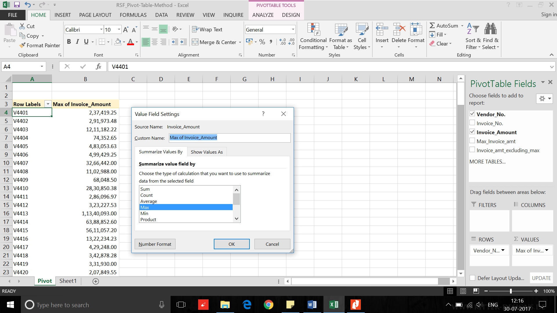
.Change the ‘Sum’ to ‘Max’ for invoice amount, this will give the maximum invoice amount for each vendor. To get maximum value go to value field setting and select summarize value by 'Max'.
Now in the data sheet using ‘VLOOKUP’ function copy the maximum invoice amount against the vendor line items in column D.
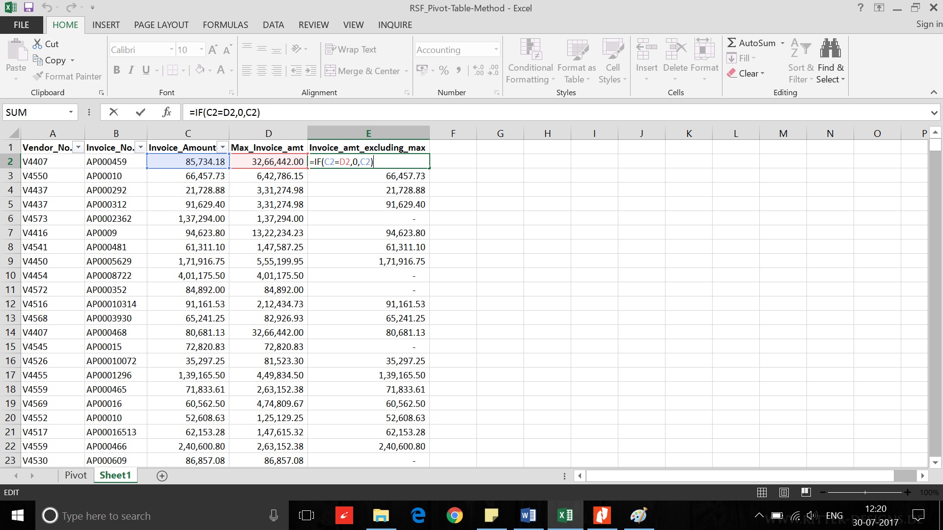
Now in column E use the “IF” formula to get invoice values. In cell E2 use this formula: E2 = IF (C2=D2,0,C2) The formula will copy all the invoice amounts except the maximum invoice amount in column E.
Now change the data source of the pivot table to include column D & E in the pivot table. To change the source go to Analyze > Change Data Source.
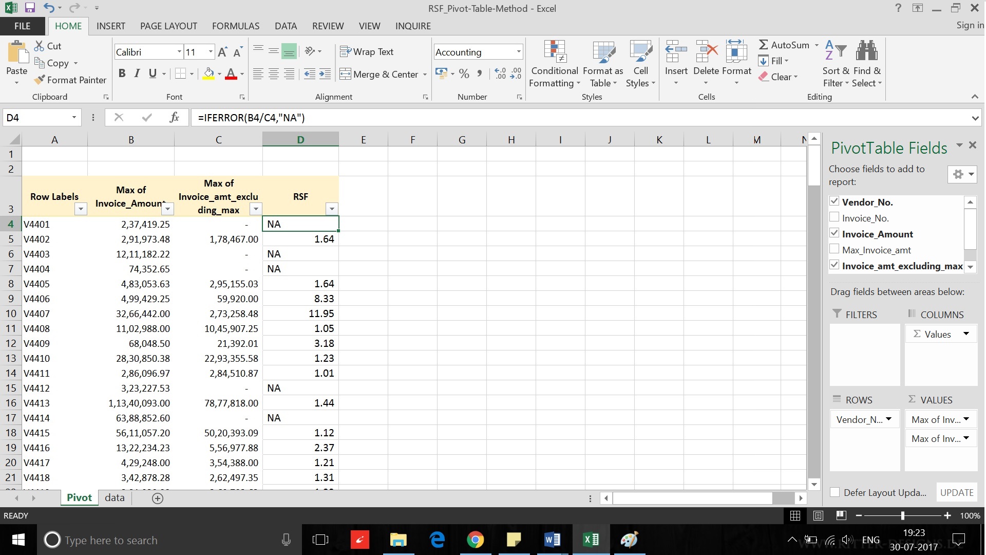
Now add the cloumn 'invoice_amt_excluding_max' (Column E) in Values and select 'Max' in the value field settings. This would give us both the largest and second largest invoice value in the Pivot table.
Calculate RSF in column D in Pivot table sheet.

Method II: Using Custom Sort and IF formula

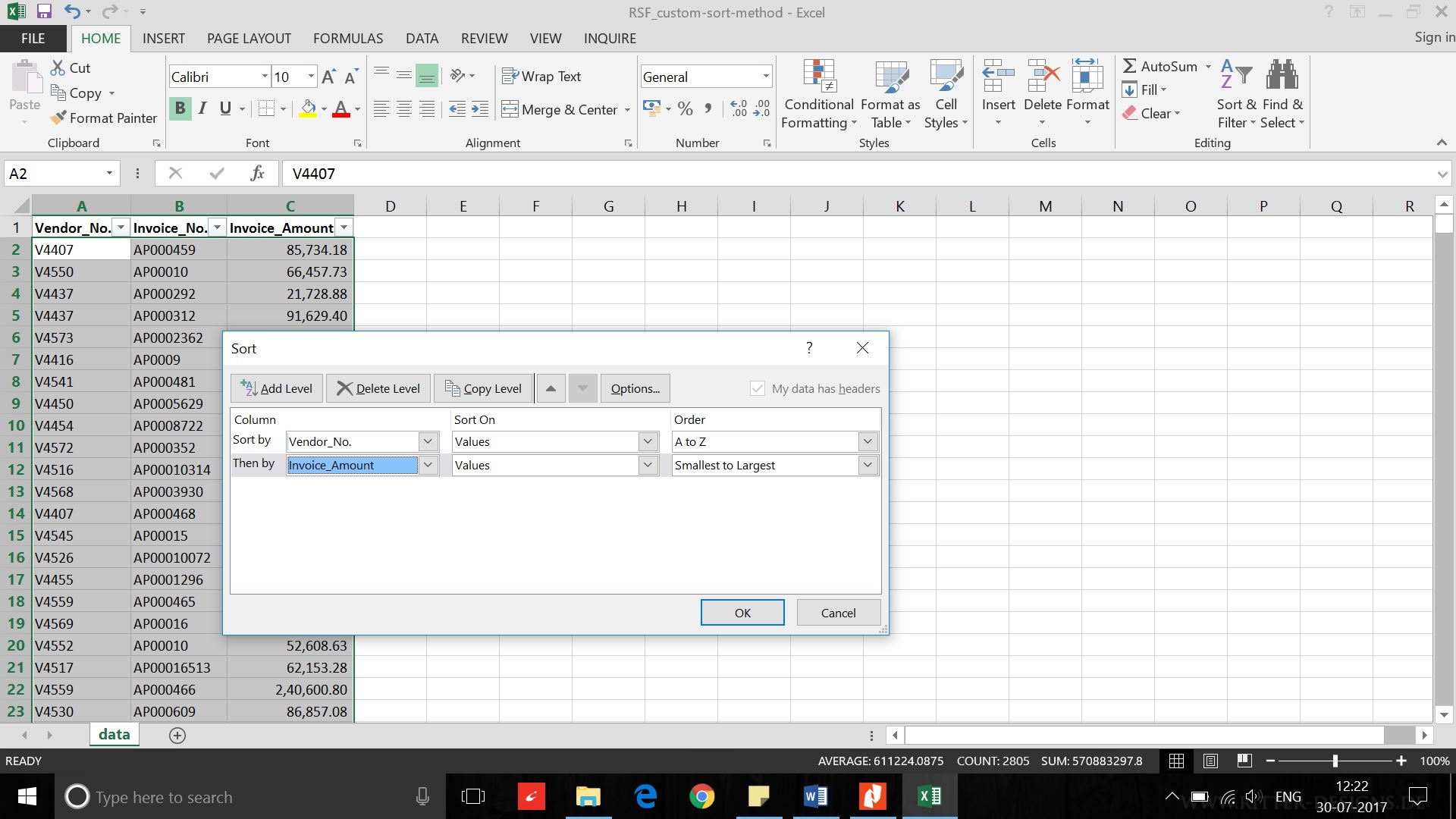
Use 'custom sort' function and sort the data with vendor number in A to Z and Invoice Amount in smallest to largest. To use 'custom sort' go to Home > Sort & Filter > Custom Sort.
In column D, use the ‘IF’ formula to get the total record count. In cell D2 put 1. In cell D3 use the following formula: D3 = If (A3=A1,D2+1,1) Copy this formula till the last record in column D. This will give the total record count for each vendor.
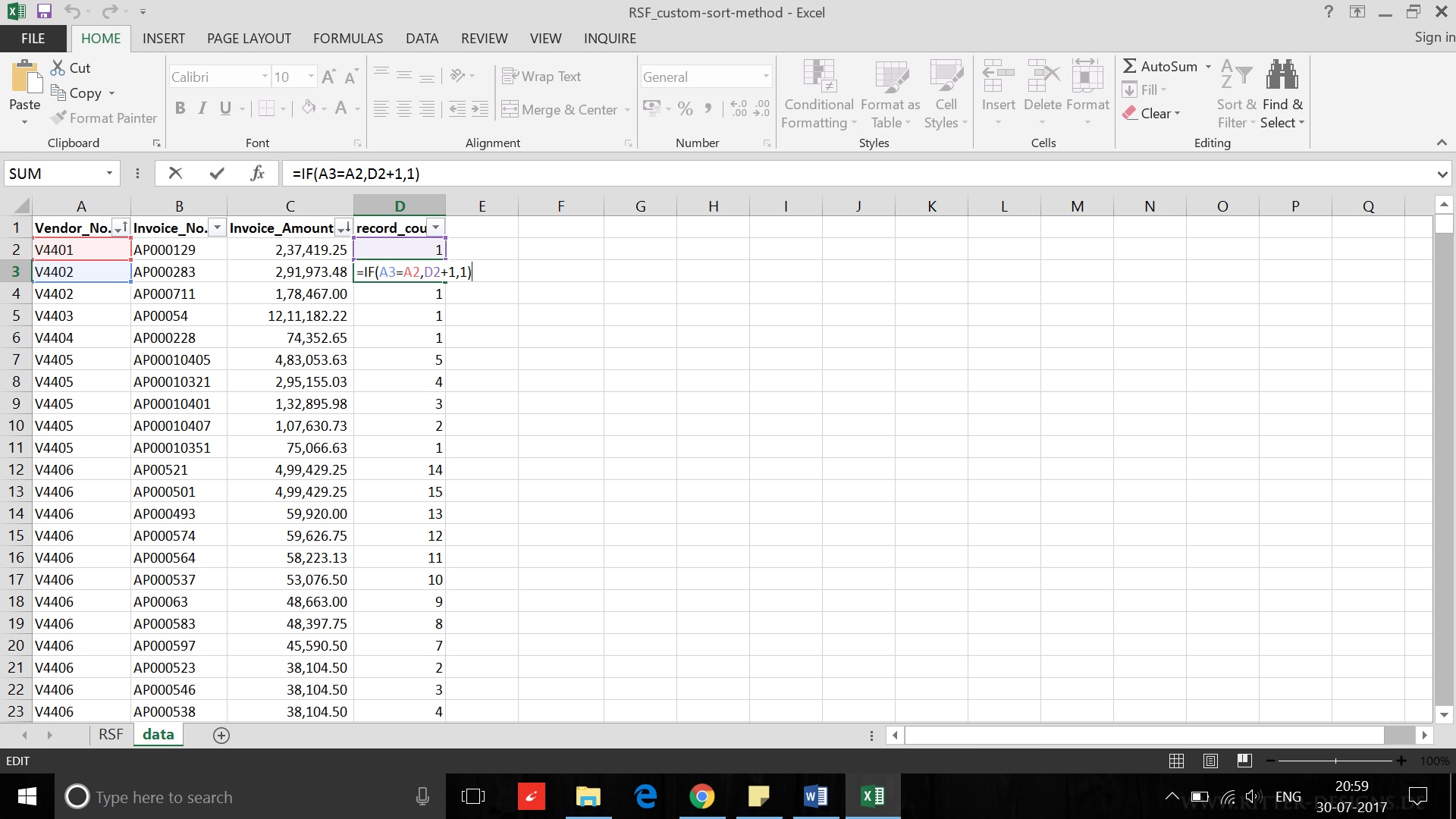
Now value paste the column D, so that the value don’t change while sorting data.
Now again use 'custom sort' and sort the data with vendor number in A to Z and Invoice Amount in largest to smallest. This will give us the largest value as first record and second largest value as second record.
Now in Column E use the same formula as used in column D. This will give us the value 1 for the largest value and 2 for the second largest value. In cell E2 put 1 and in cell E3 following formula and Copy this formula till last record in column E.; E3 = If (A3=A1,E2+1,1)
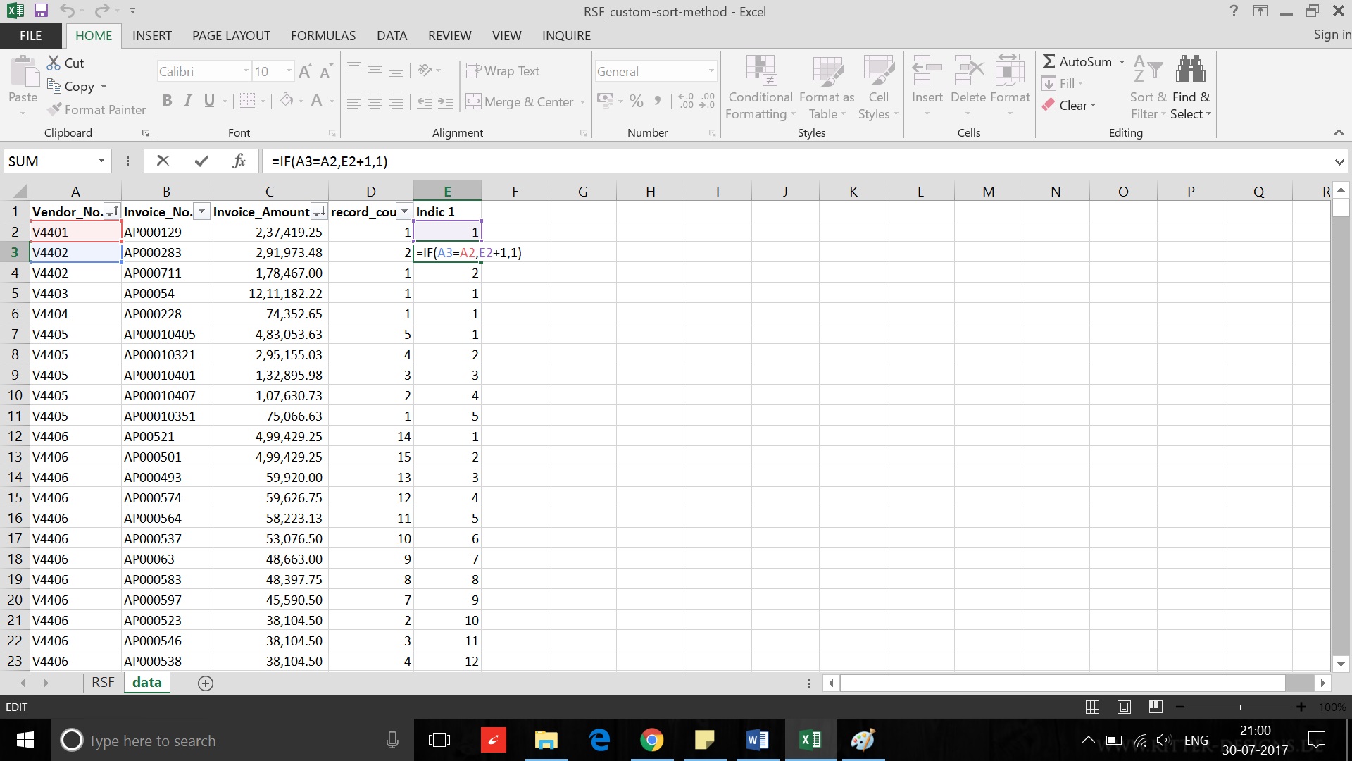
Now use a combination of ‘IF’ and ‘AND’ formula to get second largest value in the same row as that of largest value. Use the below formula starting with Cell F2; F2 = if (And (A2=A3,E3=2),C3,0) This will give the second largest number in front of largest number.
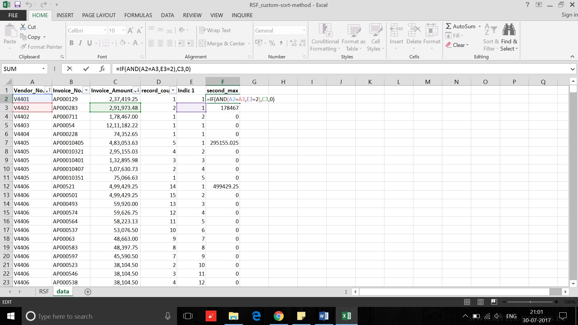
Now delete all the rows with value “0” in column F and calculate RSF for rest of the line items.

Note:

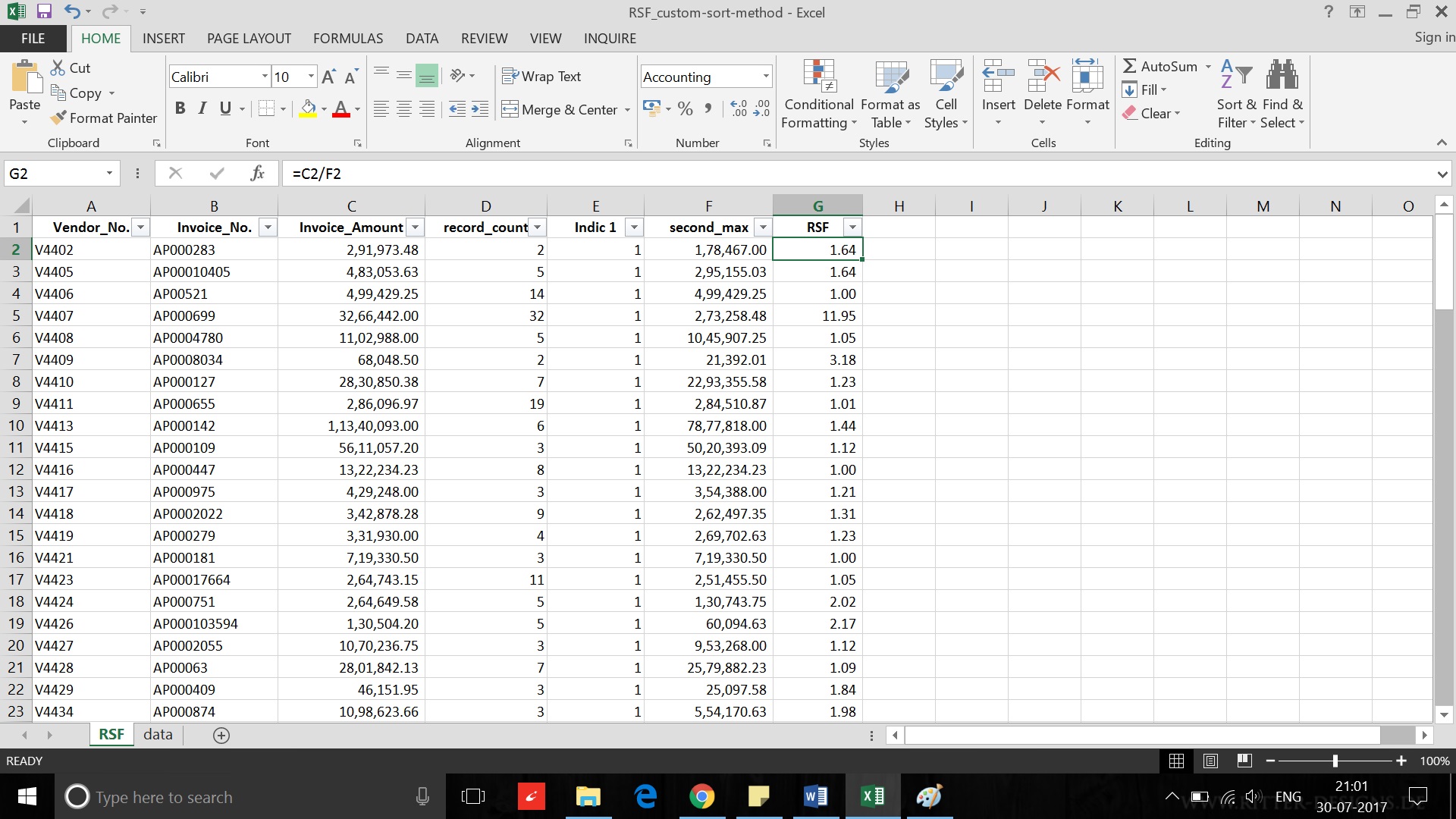
The total record count in column D, for vendors where the largest and second largest invoice amount are same, is showing one less than the actual count. For example for vendor code V4406, total records are 15 but in column D it is showing as 14 (cell D4). I’m unable to understand the reason for it.

You can download the excel files I used here, for Pivot table method , Custom Sort Method and Pivot table Filter method. If you know any other method to calculate RSF in Excel, please do let me know.

Edit 1 - 09 Sept 2017

I recently came across another method to calculate RSF in Excel using Pivot tables. Method III: Using Pivot Tables Filter Method

Create a pivot table in a new sheet. Take vendor number and invoice number in rows and invoice amount in column.
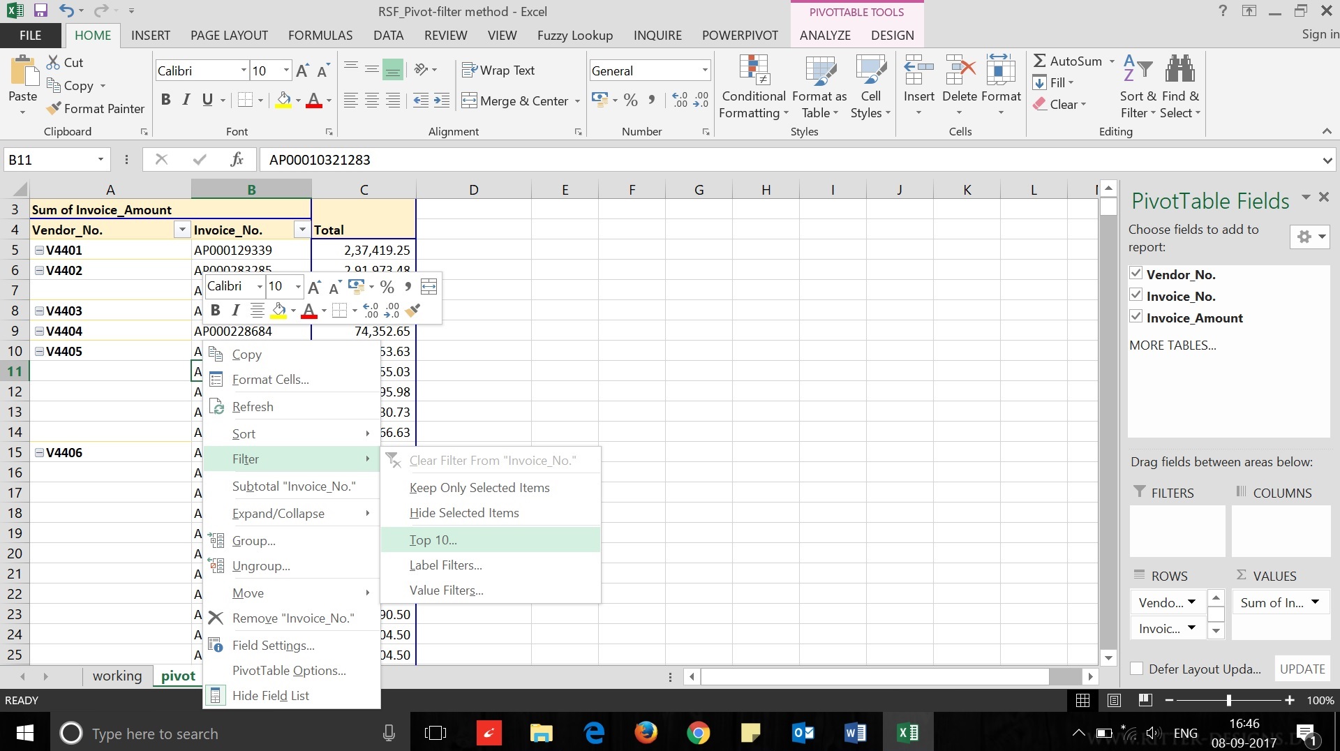
Go in any cell in Invoice Number Column. Right click, go to filter and then go to top ten items.
In the filter dialogue box select top 2 items.
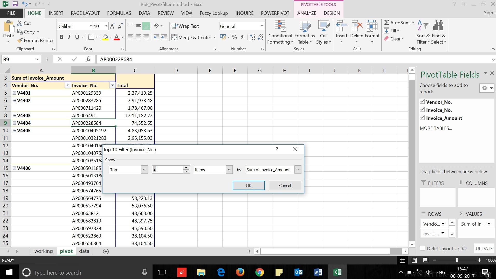
Now you will get for every vendor the top two invoice amounts. Copy this data in the new sheet.
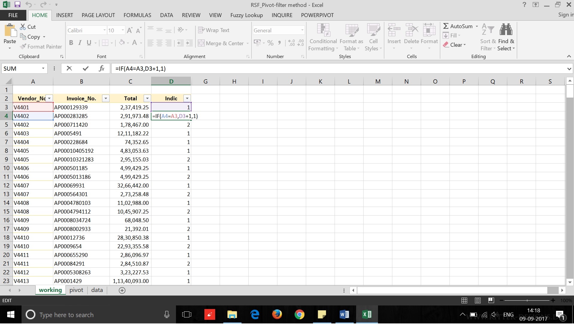
Now in Column D use the ‘IF’ formula. This formula will give us the value ‘1’ for the largest value and ‘2’ for the second largest value. In cell D3 put 1 and in cell D4 following formula; D4 = If (A4=A2,D3+1,1)
Now use a combination of ‘IF’ and ‘AND’ formula to get second largest value in the same row as that of largest value. Use the below formula starting with Cell E3; E3 = If (And (A3=A4,D4=2),C4,0)
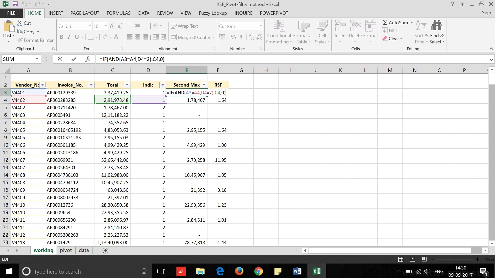
Now, in column F calculate RSF. You can delete with zero values in column E. These are the vendors only with single invoice.